Reordering columns in Excel doesn’t have to be a tedious task. Whether you’re cleaning up a dataset or preparing a report, knowing how to quickly rearrange your data can save you time and streamline your workflow.
Stick around until the end to learn how to use the MATCH formula to help align your report with another!
How To Reorder Columns in Excel
Step 1: Insert a new row above your dataset
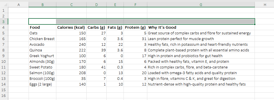
This is a simple as highlighting the header row of your data and clicking on Insert Row from within the Insert tab. If you already have a blank row above your data, you can use this.
Step 2: Index your columns
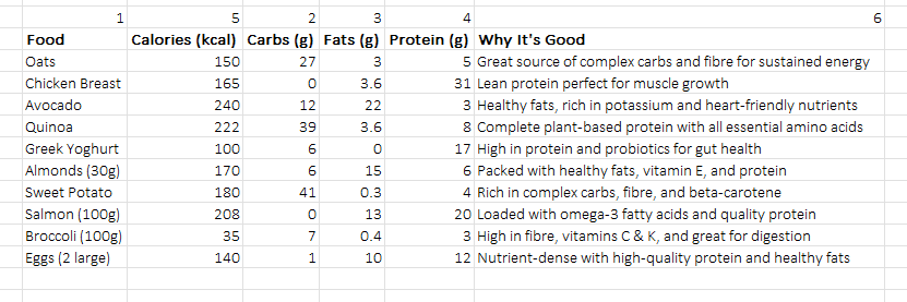
Now you have created some space, we are going to use this to add an index outlining the order we wish to see the columns appear.
For the column you wish to see first, enter the number 1 in the cell above it, for the column you wish to appear second, enter the number 2, for the third 3 and so on. If you don’t want a column to appear, leave the cell above blank. This will help us filter these out later.
In the example screenshot, we are going to get Calories to the end before the “Why It’s Good” column. In a dataset this small, you would move it manually, however the principles being shown can be translated to a larger dataset.
Step 3: Sort your columns
Most people know you can sort rows, but did you know you sort columns as well?
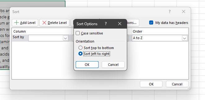
To sort your columns highlight your entire dataset and carry out the following:
- Select the Data tab and click ‘Sort’
- Click ‘options’ at the top of the pop up window and change the radio button so ‘Sort left to right’ is selected and click ok.
- Finally in the ‘Sort by’ drop down, select the row number that contains your index . The order should change to ‘Smallest to Largest’ by default. Click Ok.
![[Quickly Reorder Data Columns With Excel – select row.png]]
Step 4: Tidy up
The final thing to do is tidy up.
Begin by deleting the columns you didn’t index assuming you wish for those to be excluded from your report.
Next, remove your helper column containing your indexing, this will no longer be required.
That’s it! Your columns should now be in the order you have stated.
Bonus – Match your order to an existing report
If you need to match another report that exists already, you don’t need to index your columns manually.
Once you have created your helper row, enter the following formula above your header, assuming the first header is in cell B1:
=MATCH(B1,$A$1:$A$10,0)This formula works in the following way:
- =MATCH() – This tells excel which function we would like to call
- B1 – This is the reference of what we would like to look for. Replace this by clicking on the header you wish to search for in the document you are editing
- $A$1:$A$10 – This is the reference of the range in which you expect to see the header you are searching for appear. Assuming this range is on another tab or another document, this will be preceded by reference to that location. Make sure you lock your reference with ‘F4’ so it does not change when you drag your formula across.
- 0 – This is the way we tell the match formula we are looking for an exact match in text. This prevents any unwanted errors from lose matching.
That’s it! You will now have a reference of the position of this cell in the document you are trying to copy. You can now proceed with steps 3 and 4 as if you had manually carried out the indexing.
If this post helped get you out of a whole, please do give it a like. Knowing this content has helped somebody is the best reward for creating content!